Cold Beam in a FODO Channel with RF Cavities (and Space Charge)
This example is based on the subsection of the same name in: R. D. Ryne et al, “A Test Suite of Space-Charge Problems for Code Benchmarking”, in Proc. EPAC2004, Lucerne, Switzerland.
See additional documentation in: C. E. Mitchell et al, “ImpactX Modeling of Benchmark Tests for Space Charge Validation”, in Proc. HB2023, Geneva, Switzerland.
A cold (zero momentum spread), uniform density, 250 MeV, 143 pC proton bunch propagates in a FODO lattice with 700 MHz RF cavities added for longitudinal confinement. The on-axis profile of the RF electric field is given by:
The beam is matched to the 3D focusing, with space charge, using the rms envelope equations.
The particle distribution should remain unchanged, to within the level expected due to numerical particle noise. This is tested using the second moments of the distribution.
In this test, the initial and final values of \(\sigma_x\), \(\sigma_y\), \(\sigma_t\), \(\epsilon_x\), \(\epsilon_y\), and \(\epsilon_t\) must agree with nominal values.
Run
This example can be run either as:
Python script:
python3 run_fodo_rf_SC.pyorImpactX executable using an input file:
impactx input_fodo_rf_SC.in
For MPI-parallel runs, prefix these lines with mpiexec -n 4 ... or srun -n 4 ..., depending on the system.
#!/usr/bin/env python3
#
# Copyright 2022-2026 ImpactX contributors
# Authors: Marco Garten, Axel Huebl, Chad Mitchell
# License: BSD-3-Clause-LBNL
#
# -*- coding: utf-8 -*-

from impactx import ImpactX, distribution, elements

sim = ImpactX()

# set numerical parameters and IO control
sim.n_cell = [56, 56, 64]
sim.particle_shape = 2  # B-spline order
sim.space_charge = "3D"
sim.poisson_solver = "multigrid"
sim.dynamic_size = True
sim.prob_relative = [4.0]

# beam diagnostics
sim.slice_step_diagnostics = False

# domain decomposition & space charge mesh
sim.init_grids()

# beam parameters
kin_energy_MeV = 250.0  # reference energy
bunch_charge_C = 1.42857142857142865e-10  # used with space charge
npart = 10000  # number of macro particles

#   reference particle
ref = sim.beam.ref
ref.set_species("proton").set_kin_energy_MeV(kin_energy_MeV)

#   particle bunch
distr = distribution.Kurth6D(
    lambdaX=9.84722273e-4,
    lambdaY=6.96967278e-4,
    lambdaT=4.486799242214e-03,
    lambdaPx=0.0,
    lambdaPy=0.0,
    lambdaPt=0.0,
)
sim.add_particles(bunch_charge_C, distr, npart)

# add beam diagnostics
monitor = elements.BeamMonitor("monitor", backend="h5")

# design the accelerator lattice
sim.lattice.append(monitor)

#   Quad elements
fquad = elements.Quad(name="fquad", ds=0.15, k=2.4669749766168163, nslice=6)
dquad = elements.Quad(name="dquad", ds=0.3, k=-2.4669749766168163, nslice=12)

#   Drift element
dr = elements.Drift(name="dr", ds=0.1, nslice=4)

#   RF cavity elements
gapa1 = elements.RFCavity(
    name="gapa1",
    ds=1.0,
    escale=0.042631556991578,
    freq=7.0e8,
    phase=45.0,
    cos_coefficients=[
        0.120864178375839,
        -0.044057987631337,
        -0.209107290958498,
        -0.019831226655815,
        0.290428111491964,
        0.381974267375227,
        0.276801212694382,
        0.148265085353012,
        0.068569351192205,
        0.0290155855315696,
        0.011281649986680,
        0.004108501632832,
        0.0014277644197320,
        0.000474212125404,
        0.000151675768439,
        0.000047031436898,
        0.000014154595193,
        4.154741658e-6,
        1.191423909e-6,
        3.348293360e-7,
        9.203061700e-8,
        2.515007200e-8,
        6.478108000e-9,
        1.912531000e-9,
        2.925600000e-10,
    ],
    sin_coefficients=[
        0,
        0,
        0,
        0,
        0,
        0,
        0,
        0,
        0,
        0,
        0,
        0,
        0,
        0,
        0,
        0,
        0,
        0,
        0,
        0,
        0,
        0,
        0,
        0,
        0,
    ],
    mapsteps=100,
    nslice=4,
)

gapb1 = elements.RFCavity(
    name="gapb1",
    ds=1.0,
    escale=0.042631556991578,
    freq=7.0e8,
    phase=-1.0,
    cos_coefficients=[
        0.120864178375839,
        -0.044057987631337,
        -0.209107290958498,
        -0.019831226655815,
        0.290428111491964,
        0.381974267375227,
        0.276801212694382,
        0.148265085353012,
        0.068569351192205,
        0.0290155855315696,
        0.011281649986680,
        0.004108501632832,
        0.0014277644197320,
        0.000474212125404,
        0.000151675768439,
        0.000047031436898,
        0.000014154595193,
        4.154741658e-6,
        1.191423909e-6,
        3.348293360e-7,
        9.203061700e-8,
        2.515007200e-8,
        6.478108000e-9,
        1.912531000e-9,
        2.925600000e-10,
    ],
    sin_coefficients=[
        0,
        0,
        0,
        0,
        0,
        0,
        0,
        0,
        0,
        0,
        0,
        0,
        0,
        0,
        0,
        0,
        0,
        0,
        0,
        0,
        0,
        0,
        0,
        0,
        0,
    ],
    mapsteps=100,
    nslice=4,
)

lattice_no_drifts = [fquad, gapa1, dquad, gapb1, fquad]

#   set first lattice element
sim.lattice.append(lattice_no_drifts[0])

#   intersperse all remaining elements of the lattice with a drift element
for element in lattice_no_drifts[1:]:
    sim.lattice.extend([dr, element])

sim.lattice.append(monitor)

# run simulation
sim.track_particles()

# clean shutdown
sim.finalize()
###############################################################################
# Particle Beam(s)
###############################################################################
beam.npart = 10000
beam.units = static
beam.kin_energy = 250.0
beam.charge = 1.42857142857142865e-10
beam.particle = proton
beam.distribution = kurth6d
beam.lambdaX = 9.84722273e-4
beam.lambdaY = 6.96967278e-4
beam.lambdaT = 4.486799242214e-03
beam.lambdaPx = 0.0
beam.lambdaPy = 0.0
beam.lambdaPt = 0.0
beam.muxpx = 0.0
beam.muypy = 0.0
beam.mutpt = 0.0


###############################################################################
# Beamline: lattice elements and segments
###############################################################################
lattice.elements = monitor fquad dr gapa1 dr dquad dr gapb1 dr fquad monitor

monitor.type = beam_monitor
monitor.backend = h5

dr.type = drift
dr.ds = 0.1
dr.nslice = 4

fquad.type = quad
fquad.ds = 0.15
fquad.k = 2.4669749766168163
fquad.nslice = 6

dquad.type = quad
dquad.ds = 0.3
dquad.k = -fquad.k
dquad.nslice = 12

gapa1.type = rfcavity
gapa1.ds = 1.0
gapa1.escale = 0.042631556991578
gapa1.freq = 7.0e8
gapa1.phase = 45.0
gapa1.mapsteps = 100
gapa1.nslice = 10
gapa1.cos_coefficients =           \
                0.120864178375839  \
                -0.044057987631337 \
                -0.209107290958498 \
                -0.019831226655815 \
                0.290428111491964  \
                0.381974267375227  \
                0.276801212694382  \
                0.148265085353012  \
                0.068569351192205  \
                0.0290155855315696 \
                0.011281649986680  \
                0.004108501632832  \
                0.0014277644197320 \
                0.000474212125404  \
                0.000151675768439  \
                0.000047031436898  \
                0.000014154595193  \
                4.154741658e-6     \
                1.191423909e-6     \
                3.348293360e-7     \
                9.203061700e-8     \
                2.515007200e-8     \
                6.478108000e-9     \
                1.912531000e-9     \
                2.925600000e-10
gapa1.sin_coefficients = 0 0 0 0 0 0 0 0 0 0 0 0 0 0 0 0 0 0  \
                0 0 0 0 0 0 0

gapb1.type = rfcavity
gapb1.ds = 1.0
gapb1.escale = 0.042631556991578
gapb1.freq = 7.0e8
gapb1.phase = -1.0
gapb1.mapsteps = 100
gapb1.nslice = 10
gapb1.cos_coefficients =            \
                0.120864178375839   \
                -0.044057987631337  \
                -0.209107290958498  \
                -0.019831226655815  \
                0.290428111491964   \
                0.381974267375227   \
                0.276801212694382   \
                0.148265085353012   \
                0.068569351192205   \
                0.0290155855315696  \
                0.011281649986680   \
                0.004108501632832   \
                0.0014277644197320  \
                0.000474212125404   \
                0.000151675768439   \
                0.000047031436898   \
                0.000014154595193   \
                4.154741658e-6      \
                1.191423909e-6      \
                3.348293360e-7      \
                9.203061700e-8      \
                2.515007200e-8      \
                6.478108000e-9      \
                1.912531000e-9      \
                2.925600000e-10
gapb1.sin_coefficients = 0 0 0 0 0 0 0 0 0 0 0 0 0 0 0 0 0 0  \
                0 0 0 0 0 0 0


###############################################################################
# Algorithms
###############################################################################
algo.particle_shape = 2
algo.space_charge = 3D
algo.poisson_solver = "multigrid"

amr.n_cell = 56 56 64
geometry.prob_relative = 4.0

###############################################################################
# Diagnostics
###############################################################################
diag.slice_step_diagnostics = false
Analyze
We run the following script to analyze correctness:
Script analysis_fodo_rf_SC.py
#!/usr/bin/env python3
#
# Copyright 2022-2026 ImpactX contributors
# Authors: Axel Huebl, Chad Mitchell
# License: BSD-3-Clause-LBNL
#

import numpy as np
import openpmd_api as io
from scipy.stats import moment


def get_moments(beam):
    """Calculate standard deviations of beam position & momenta
    and emittance values

    Returns
    -------
    sigx, sigy, sigt, emittance_x, emittance_y, emittance_t
    """
    sigx = moment(beam["position_x"], moment=2) ** 0.5  # variance -> std dev.
    sigpx = moment(beam["momentum_x"], moment=2) ** 0.5
    sigy = moment(beam["position_y"], moment=2) ** 0.5
    sigpy = moment(beam["momentum_y"], moment=2) ** 0.5
    sigt = moment(beam["position_t"], moment=2) ** 0.5
    sigpt = moment(beam["momentum_t"], moment=2) ** 0.5

    epstrms = beam.cov(ddof=0)
    emittance_x = (sigx**2 * sigpx**2 - epstrms["position_x"]["momentum_x"] ** 2) ** 0.5
    emittance_y = (sigy**2 * sigpy**2 - epstrms["position_y"]["momentum_y"] ** 2) ** 0.5
    emittance_t = (sigt**2 * sigpt**2 - epstrms["position_t"]["momentum_t"] ** 2) ** 0.5

    return (sigx, sigy, sigt, emittance_x, emittance_y, emittance_t)


# initial/final beam
series = io.Series("diags/openPMD/monitor.h5", io.Access.read_only)
last_step = list(series.iterations)[-1]
initial = series.iterations[1].particles["beam"].to_df()
final = series.iterations[last_step].particles["beam"].to_df()

# compare number of particles
num_particles = 10000
assert num_particles == len(initial)
assert num_particles == len(final)

print("Initial Beam:")
sigx, sigy, sigt, emittance_x, emittance_y, emittance_t = get_moments(initial)
print(f"  sigx={sigx:e} sigy={sigy:e} sigt={sigt:e}")

atol = 0.0  # ignored
rtol = 3.0 * num_particles**-0.5  # from random sampling of a smooth distribution
print(f"  rtol={rtol} (ignored: atol~={atol})")

assert np.allclose(
    [sigx, sigy, sigt],
    [9.84722273e-4, 6.96967278e-4, 4.486799242214e-03],
    rtol=rtol,
    atol=atol,
)

print(
    f"  emittance_x={emittance_x:e} emittance_y={emittance_y:e} emittance_t={emittance_t:e}"
)

atol = 4.0e-8
print(f"  atol={atol}")

assert np.allclose(
    [emittance_x, emittance_y, emittance_t],
    [0.0, 0.0, 0.0],
    atol=atol,
)


print("")
print("Final Beam:")
sigx, sigy, sigt, emittance_x, emittance_y, emittance_t = get_moments(final)
print(f"  sigx={sigx:e} sigy={sigy:e} sigt={sigt:e}")

atol = 0.0  # ignored
rtol = 3.6 * num_particles**-0.5  # from random sampling of a smooth distribution
print(f"  rtol={rtol} (ignored: atol~={atol})")

assert np.allclose(
    [sigx, sigy, sigt],
    [9.84722273e-4, 6.96967278e-4, 4.486799242214e-03],
    rtol=rtol,
    atol=atol,
)

print(
    f"  emittance_x={emittance_x:e} emittance_y={emittance_y:e} emittance_t={emittance_t:e}"
)

atol = 4.0e-8
print(f"  atol={atol}")

assert np.allclose(
    [emittance_x, emittance_y, emittance_t],
    [0.0, 0.0, 0.0],
    atol=atol,
)
Thermal Beam in a Constant Focusing Channel (with Space Charge)
This example is based on the subsection of the same name in: R. D. Ryne et al, “A Test Suite of Space-Charge Problems for Code Benchmarking”, in Proc. EPAC2004, Lucerne, Switzerland.
See additional documentation in: C. E. Mitchell et al, “ImpactX Modeling of Benchmark Tests for Space Charge Validation”, in Proc. HB2023, Geneva, Switzerland.
This example illustrates a stationary solution of the Vlasov-Poisson equations with spherical symmetry (in the beam rest frame). The distribution represents a thermal equilibrium of the form:
where \(C\) and \(kT\) are constants, and \(H\) denotes the self-consistent Hamiltonian with space charge.
In this example, a 0.1 MeV, 143 pC proton bunch with \(kT=36\times 10^{-6}\) propagates in a constant focusing lattice with 3D isotropic focusing. (The isotropy is exact in the beam rest frame.)
The particle distribution should remain unchanged, to within the level expected due to numerical particle noise. This is tested using the second moments of the distribution.
In this test, the initial and final values of \(\sigma_x\), \(\sigma_y\), \(\sigma_t\), \(\epsilon_x\), \(\epsilon_y\), and \(\epsilon_t\) must agree with nominal values.
Run
This example can be run either as:
Python script:
python3 run_thermal.pyorImpactX executable using an input file:
impactx input_thermal.in
For MPI-parallel runs, prefix these lines with mpiexec -n 4 ... or srun -n 4 ..., depending on the system.
#!/usr/bin/env python3
#
# Copyright 2022-2026 ImpactX contributors
# Authors: Marco Garten, Axel Huebl, Chad Mitchell
# License: BSD-3-Clause-LBNL
#
# -*- coding: utf-8 -*-

from impactx import ImpactX, distribution, elements

sim = ImpactX()

# set numerical parameters and IO control
sim.n_cell = [56, 56, 64]
sim.particle_shape = 2  # B-spline order
sim.space_charge = "3D"
sim.dynamic_size = True
sim.prob_relative = [4.0]

# beam diagnostics
sim.slice_step_diagnostics = False

# domain decomposition & space charge mesh
sim.init_grids()

# beam parameters
kin_energy_MeV = 0.1  # reference energy
bunch_charge_C = 1.4285714285714285714e-10  # used with space charge
npart = 10000  # number of macro particles

#   reference particle
ref = sim.beam.ref
ref.set_species("proton").set_kin_energy_MeV(kin_energy_MeV)

#   particle bunch
distr = distribution.Thermal(
    k=6.283185307179586,
    kT=36.0e-6,
    kT_halo=36.0e-6,
    normalize=0.41604661,
    normalize_halo=0.0,
    w_halo=0.0,
)
sim.add_particles(bunch_charge_C, distr, npart)

# add beam diagnostics
monitor = elements.BeamMonitor("monitor", backend="h5")

# design the accelerator lattice
sim.lattice.append(monitor)

constf = elements.Constf(
    ds=10.0,
    kx=6.283185307179586,
    ky=6.283185307179586,
    kt=6.283185307179586,
    nslice=400,
)

#   set first lattice element
sim.lattice.append(constf)
sim.lattice.append(monitor)

# run simulation
sim.track_particles()

# clean shutdown
sim.finalize()
###############################################################################
# Particle Beam(s)
###############################################################################
#beam.npart = 100000000  #full resolution
beam.npart = 10000
beam.units = static
beam.kin_energy = 0.1
beam.charge = 1.4285714285714285714e-10
beam.particle = proton
beam.distribution = thermal
beam.k = 6.283185307179586
beam.kT = 36.0e-6
beam.normalize = 0.41604661

###############################################################################
# Beamline: lattice elements and segments
###############################################################################
lattice.elements = monitor constf1 monitor

monitor.type = beam_monitor
monitor.backend = h5

constf1.type = constf
constf1.ds = 10.0
constf1.kx = 6.283185307179586
constf1.ky = constf1.kx
constf1.kt = constf1.kx
constf1.nslice = 400   #full resolution
#constf1.nslice = 50


###############################################################################
# Algorithms
###############################################################################
algo.particle_shape = 2
algo.space_charge = 3D

#amr.n_cell = 128 128 128  #full resolution
amr.n_cell = 64 64 64
geometry.prob_relative = 3.0

###############################################################################
# Diagnostics
###############################################################################
diag.slice_step_diagnostics = false
Analyze
We run the following script to analyze correctness:
Script analysis_thermal.py
#!/usr/bin/env python3
#
# Copyright 2022-2026 ImpactX contributors
# Authors: Axel Huebl, Chad Mitchell
# License: BSD-3-Clause-LBNL
#


import numpy as np
import openpmd_api as io
from scipy.stats import moment


def get_moments(beam):
    """Calculate standard deviations of beam position & momenta
    and emittance values

    Returns
    -------
    sigx, sigy, sigt, emittance_x, emittance_y, emittance_t
    """
    sigx = moment(beam["position_x"], moment=2) ** 0.5  # variance -> std dev.
    sigpx = moment(beam["momentum_x"], moment=2) ** 0.5
    sigy = moment(beam["position_y"], moment=2) ** 0.5
    sigpy = moment(beam["momentum_y"], moment=2) ** 0.5
    sigt = moment(beam["position_t"], moment=2) ** 0.5
    sigpt = moment(beam["momentum_t"], moment=2) ** 0.5

    epstrms = beam.cov(ddof=0)
    emittance_x = (sigx**2 * sigpx**2 - epstrms["position_x"]["momentum_x"] ** 2) ** 0.5
    emittance_y = (sigy**2 * sigpy**2 - epstrms["position_y"]["momentum_y"] ** 2) ** 0.5
    emittance_t = (sigt**2 * sigpt**2 - epstrms["position_t"]["momentum_t"] ** 2) ** 0.5

    return (sigx, sigy, sigt, emittance_x, emittance_y, emittance_t)


# initial/final beam
series = io.Series("diags/openPMD/monitor.h5", io.Access.read_only)
last_step = list(series.iterations)[-1]
initial = series.iterations[1].particles["beam"].to_df()
final = series.iterations[last_step].particles["beam"].to_df()

# compare number of particles
num_particles = 10000
assert num_particles == len(initial)
assert num_particles == len(final)

print("Initial Beam:")
sigx, sigy, sigt, emittance_x, emittance_y, emittance_t = get_moments(initial)
print(f"  sigx={sigx:e} sigy={sigy:e} sigt={sigt:e}")
print(
    f"  emittance_x={emittance_x:e} emittance_y={emittance_y:e} emittance_t={emittance_t:e}"
)

atol = 0.0  # ignored
rtol = 3.5 * num_particles**-0.5  # from random sampling of a smooth distribution
print(f"  rtol={rtol} (ignored: atol~={atol})")

assert np.allclose(
    [sigx, sigy, sigt, emittance_x, emittance_y, emittance_t],
    [
        2.569162e-03,
        2.569557e-03,
        1.757951e-01,
        1.540773e-05,
        1.541883e-05,
        1.538814e-05,
    ],
    rtol=rtol,
    atol=atol,
)


print("")
print("Final Beam:")
sigx, sigy, sigt, emittance_x, emittance_y, emittance_t = get_moments(final)
print(f"  sigx={sigx:e} sigy={sigy:e} sigt={sigt:e}")
print(
    f"  emittance_x={emittance_x:e} emittance_y={emittance_y:e} emittance_t={emittance_t:e}"
)

atol = 0.0  # ignored
rtol = 6.0 * num_particles**-0.5  # from random sampling of a smooth distribution
print(f"  rtol={rtol} (ignored: atol~={atol})")

assert np.allclose(
    [sigx, sigy, sigt, emittance_x, emittance_y, emittance_t],
    [
        2.569162e-03,
        2.569557e-03,
        1.757951e-01,
        1.540773e-05,
        1.541883e-05,
        1.538814e-05,
    ],
    rtol=rtol,
    atol=atol,
)
Bithermal Beam in a Constant Focusing Channel (with Space Charge)
This example is based on the subsection of the same name in: R. D. Ryne et al, “A Test Suite of Space-Charge Problems for Code Benchmarking”, in Proc. EPAC2004, Lucerne, Switzerland.
See additional documentation in: C. E. Mitchell et al, “ImpactX Modeling of Benchmark Tests for Space Charge Validation”, in Proc. HB2023, Geneva, Switzerland.
This example illustrates a stationary solution of the Vlasov-Poisson equations with spherical symmetry (in the beam rest frame). It provides a self-consistent model of a 3D bunch with a nontrivial core-halo distribution.
The distribution represents a bithermal stationary distribution of the form:
where \(c_j\), \(kT_j\) \((j=1,2)\) are constants, and \(H\) denotes the self-consistent Hamiltonian with space charge.
In this example, a 0.1 MeV, 143 pC proton bunch with \(kT_1=36\times 10^{-6}\) and \(kT_1=900\times 10^{-6}\) propagates in a constant focusing lattice with 3D isotropic focusing. (The isotropy is exact in the beam rest frame.) 5% of the total charge lies in the second (halo) population.
The particle distribution should remain unchanged, to within the level expected due to numerical particle noise. This is tested using the second moments of the distribution.
In this test, the initial and final values of \(\sigma_x\), \(\sigma_y\), \(\sigma_t\), \(\epsilon_x\), \(\epsilon_y\), and \(\epsilon_t\) must agree with nominal values.
Run
This example can be run either as:
Python script:
python3 run_bithermal.pyorImpactX executable using an input file:
impactx input_bithermal.in
For MPI-parallel runs, prefix these lines with mpiexec -n 4 ... or srun -n 4 ..., depending on the system.
#!/usr/bin/env python3
#
# Copyright 2022-2026 ImpactX contributors
# Authors: Marco Garten, Axel Huebl, Chad Mitchell
# License: BSD-3-Clause-LBNL
#
# -*- coding: utf-8 -*-

from impactx import ImpactX, distribution, elements

sim = ImpactX()

# set numerical parameters and IO control
sim.n_cell = [64, 64, 64]
sim.particle_shape = 2  # B-spline order
sim.space_charge = "3D"
sim.poisson_solver = "fft"
sim.dynamic_size = True
sim.prob_relative = [1.1]

# beam diagnostics
sim.slice_step_diagnostics = False

# domain decomposition & space charge mesh
sim.init_grids()

# beam parameters
kin_energy_MeV = 0.1  # reference energy
bunch_charge_C = 1.4285714285714285714e-10  # used with space charge
# npart = 1000000  # full resolution
npart = 10000

#   reference particle
ref = sim.beam.ref
ref.set_species("proton").set_kin_energy_MeV(kin_energy_MeV)

#   particle bunch
distr = distribution.Thermal(
    k=6.283185307179586,
    kT=36.0e-6,
    kT_halo=900.0e-6,
    normalize=0.54226,
    normalize_halo=0.08195,
    halo=0.05,
)
sim.add_particles(bunch_charge_C, distr, npart)

# add beam diagnostics
monitor = elements.BeamMonitor("monitor", backend="h5")

# design the accelerator lattice
sim.lattice.append(monitor)

constf = elements.ConstF(
    name="constf",
    ds=10.0,
    kx=6.283185307179586,
    ky=6.283185307179586,
    kt=6.283185307179586,
    # nslice=400,  # full resolution
    nslice=120,
)

sim.lattice.append(constf)
sim.lattice.append(monitor)

# run simulation
sim.track_particles()

# clean shutdown
sim.finalize()
###############################################################################
# Particle Beam(s)
###############################################################################
#beam.npart = 1000000  #full resolution
beam.npart = 10000
beam.units = static
beam.kin_energy = 0.1
beam.charge = 1.4285714285714285714e-10
beam.particle = proton
beam.distribution = thermal
beam.k = 6.283185307179586
beam.kT = 36.0e-6
beam.kT_halo = 900.0e-6
beam.halo = 0.05
beam.normalize = 0.54226
beam.normalize_halo = 0.08195


###############################################################################
# Beamline: lattice elements and segments
###############################################################################
lattice.elements = monitor constf1 monitor

monitor.type = beam_monitor
monitor.backend = h5

constf1.type = constf
constf1.ds = 10.0
constf1.kx = 6.283185307179586
constf1.ky = constf1.kx
constf1.kt = constf1.kx
#constf1.nslice = 400  #full resolution
constf1.nslice = 120

###############################################################################
# Algorithms
###############################################################################
algo.particle_shape = 2
algo.space_charge = 3D
algo.poisson_solver = "fft"

amr.n_cell = 64 64 64
geometry.prob_relative = 1.1

###############################################################################
# Diagnostics
###############################################################################
diag.slice_step_diagnostics = false
Analyze
We run the following script to analyze correctness:
Script analysis_bithermal.py
#!/usr/bin/env python3
#
# Copyright 2022-2026 ImpactX contributors
# Authors: Axel Huebl, Chad Mitchell
# License: BSD-3-Clause-LBNL
#


import numpy as np
import openpmd_api as io
from scipy.stats import moment


def get_moments(beam):
    """Calculate standard deviations of beam position & momenta
    and emittance values

    Returns
    -------
    sigx, sigy, sigt, emittance_x, emittance_y, emittance_t
    """
    sigx = moment(beam["position_x"], moment=2) ** 0.5  # variance -> std dev.
    sigpx = moment(beam["momentum_x"], moment=2) ** 0.5
    sigy = moment(beam["position_y"], moment=2) ** 0.5
    sigpy = moment(beam["momentum_y"], moment=2) ** 0.5
    sigt = moment(beam["position_t"], moment=2) ** 0.5
    sigpt = moment(beam["momentum_t"], moment=2) ** 0.5

    epstrms = beam.cov(ddof=0)
    emittance_x = (sigx**2 * sigpx**2 - epstrms["position_x"]["momentum_x"] ** 2) ** 0.5
    emittance_y = (sigy**2 * sigpy**2 - epstrms["position_y"]["momentum_y"] ** 2) ** 0.5
    emittance_t = (sigt**2 * sigpt**2 - epstrms["position_t"]["momentum_t"] ** 2) ** 0.5

    return (sigx, sigy, sigt, emittance_x, emittance_y, emittance_t)


# initial/final beam
series = io.Series("diags/openPMD/monitor.h5", io.Access.read_only)
last_step = list(series.iterations)[-1]
initial = series.iterations[1].particles["beam"].to_df()
final = series.iterations[last_step].particles["beam"].to_df()

# compare number of particles
num_particles = 10000
assert num_particles == len(initial)
assert num_particles == len(final)

print("Initial Beam:")
sigx, sigy, sigt, emittance_x, emittance_y, emittance_t = get_moments(initial)
print(f"  sigx={sigx:e} sigy={sigy:e} sigt={sigt:e}")
print(
    f"  emittance_x={emittance_x:e} emittance_y={emittance_y:e} emittance_t={emittance_t:e}"
)

atol = 0.0  # ignored
rtol = 4.0 * num_particles**-0.5  # from random sampling of a smooth distribution
print(f"  rtol={rtol} (ignored: atol~={atol})")

assert np.allclose(
    [sigx, sigy, sigt, emittance_x, emittance_y, emittance_t],
    [
        2.751162e-03,
        2.751725e-03,
        1.884003e-01,
        2.449966e-05,
        2.451077e-05,
        2.444195e-05,
    ],
    rtol=rtol,
    atol=atol,
)


print("")
print("Final Beam:")
sigx, sigy, sigt, emittance_x, emittance_y, emittance_t = get_moments(final)
print(f"  sigx={sigx:e} sigy={sigy:e} sigt={sigt:e}")
print(
    f"  emittance_x={emittance_x:e} emittance_y={emittance_y:e} emittance_t={emittance_t:e}"
)

atol = 0.0  # ignored
rtol = 0.07  # dominated by space-charge modeling, not particle sampling
print(f"  rtol={rtol} (ignored: atol~={atol})")

assert np.allclose(
    [sigx, sigy, sigt, emittance_x, emittance_y, emittance_t],
    [
        2.751162e-03,
        2.751725e-03,
        1.884003e-01,
        2.449966e-05,
        2.451077e-05,
        2.444195e-05,
    ],
    rtol=rtol,
    atol=atol,
)
Visualize
You can run the following script to visualize the initial and final beam distribution:
Script plot_bithermal.py
#!/usr/bin/env python3
#
# Copyright 2022-2026 ImpactX contributors
# Authors: Axel Huebl, Chad Mitchell
# License: BSD-3-Clause-LBNL
#

import argparse
from math import pi

import matplotlib.pyplot as plt
import numpy as np
import openpmd_api as io

# options to run this script
parser = argparse.ArgumentParser(description="Plot the Bithermal benchmark.")
parser.add_argument(
    "--save-png", action="store_true", help="non-interactive run: save to PNGs"
)
args = parser.parse_args()


# initial/final beam
series = io.Series("diags/openPMD/monitor.h5", io.Access.read_only)
last_step = list(series.iterations)[-1]
initial_beam = series.iterations[1].particles["beam"].to_df()
final_beam = series.iterations[last_step].particles["beam"].to_df()

# Constants
w1 = 0.95
w2 = 0.05
bg = 0.0146003
Min = 0.0
Max = 0.025
Np = 100000001
n = 300


# Function for radius calculation
def r(x, y, z):
    return np.sqrt(x**2 + y**2 + z**2)


# Calculate radius and bin data
initial_radii = r(
    bg * initial_beam["position_t"],
    initial_beam["position_x"],
    initial_beam["position_y"],
)
initial_hist, bin_edges = np.histogram(initial_radii, bins=n, range=(Min, Max))
initial_bin_centers = 0.5 * (bin_edges[:-1] + bin_edges[1:])

final_radii = r(
    bg * final_beam["position_t"], final_beam["position_x"], final_beam["position_y"]
)
final_hist, _ = np.histogram(final_radii, bins=n, range=(Min, Max))

# dr (m)
initial_r = initial_hist / (Np * (bin_edges[1] - bin_edges[0]))
final_r = final_hist / (Np * (bin_edges[1] - bin_edges[0]))

# Plotting
plt.figure(figsize=(10, 6))
plt.xscale("linear")
plt.yscale("log")
plt.xlim([Min, Max])
plt.ylim([0.1, 1.6e6])
plt.xlabel("r (m)", fontsize=30)
plt.xticks(fontsize=25)
plt.yticks(fontsize=25)
plt.grid(True)

# Plot the data
plt.plot(
    initial_bin_centers,
    initial_r / (4.0 * pi * (initial_bin_centers) ** 2),
    label="Initial beam",
    linewidth=2,
)
plt.plot(
    initial_bin_centers,
    final_r / (4.0 * pi * (initial_bin_centers) ** 2),
    label="Final beam",
    linewidth=2,
    linestyle="dotted",
)

# Show plot
plt.legend(fontsize=20)

plt.tight_layout()
if args.save_png:
    plt.savefig("bithermal.png")
else:
    plt.show()
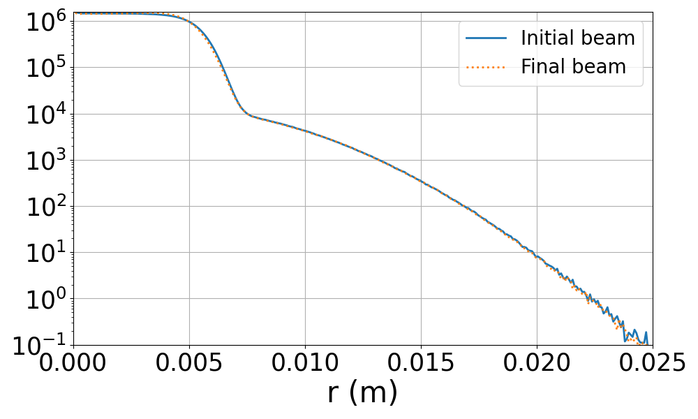
Fig. 10 Initial and final beam distribution when running with full resolution (see inline comments in the input file/script). The bithermal distribution should stay static in this test.